A PBGL Quantitative Locus and Bulk Segregant Analysis in R Sorghum Semi-dwarfism
Software Prerequisites in an Environment .YAML Form
name: QTLseqr

channels:
- default
- bioconda
- conda-forge
- r

dependencies:
- r-modeest >= 2.3.2
- r-ggplot2 >= 2.2.0
- r-gtools
- r-dplyr
- r-readr
- r-tidyr
- r-Rcpp
- r-locfit
- r-knitr
- r-rmarkdown
- r-kableExtra
- r-devtools
- r-data.table
- r-vcfR
- r-optparse
- r-base >= 4.1.0
Install manually in RStudio
#install the dependencies
install.packages(c("data.table",
           "modeest",
           "locfit",
           "dplyr",
           "tidyr",
           "vcfR",
           "ggplot2"), dependencies=TRUE)

# install devtools
install.packages("devtools", dependencies=TRUE)

# use devtools to install QTLseqr from github
library("devtools")
#devtools::install_github("bmansfeld/QTLseqr")
#devtools::install_github("warthmann/QTLseqr")
devtools::install_github("pbgl/QTLseqr")


#load dependencies
library("devtools")
library("data.table")
library("dplyr")
library("tidyr")
library("vcfR")
library("ggplot2")

#load the package
library("QTLseqr")
Data Analysis
Import VCF
QTLseqr::importFromVCF(file = "freebayes_D2.filtered.vcf",highBulk = "D2_F2_tt",lowBulk = "D2_F2_TT",
chromList = c("Chr01","Chr02","Chr03","Chr04","Chr05","Chr06","Chr07","Chr08","Chr09","Chr10"),
,filter=FALSE, outfile=TRUE)
#Set High bulk and Low bulk sample names and parser generated file name
#The file name is generated from the QTLParser_1_MH function in line 119
Filter SNPs
     #Filter SNPs based on some criteria
     df_filt <-
 QTLseqr::filterSNPs(
 SNPset = df,
 refAlleleFreq = 0.20,
 minTotalDepth = 100,
 maxTotalDepth = 400,
 minSampleDepth = 40,
          minGQ = 99,
 verbose = TRUE
)
G Prime Analysis
    #Run G' analysis
    df_filt<-QTLseqr::runGprimeAnalysis(
SNPset = df_filt,
windowSize = 5000000,
outlierFilter = "deltaSNP",
filterThreshold = 0.1)
QTLseq Analysis
    #Run QTLseq analysis
    df_filt <- QTLseqr::runQTLseqAnalysis(
SNPset = df_filt,
windowSize = 5000000,
popStruc = "F2",
bulkSize = c(45, 38),
replications = 10000,
intervals = c(95, 99)
    )
QTL Peak Mapping
#Plot
QTLseqr::plotQTLStats(SNPset = df_filt, var = "Gprime", plotThreshold = TRUE, q = 0.01)
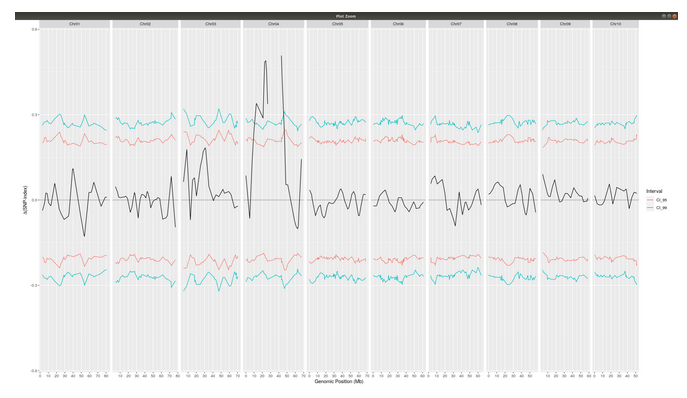
QTLseqr::plotQTLStats(SNPset = df_filt, var = "deltaSNP", plotIntervals  = TRUE)

#export summary CSV
QTLseqr::getQTLTable(SNPset = df_filt, alpha = 0.01, export = TRUE, fileName = "my_BSA_QTL.csv")

High Impact Variants QTL1 on Chromosome 4
df <- df_filt %>% dplyr::filter(CHROM=="Chr04")
df <- df %>% dplyr::filter(POS >= 1757999 & POS <= 46793997)
write.table(df, file = "HighImpactVariants.txt", row.names = FALSE)

Plotting Images
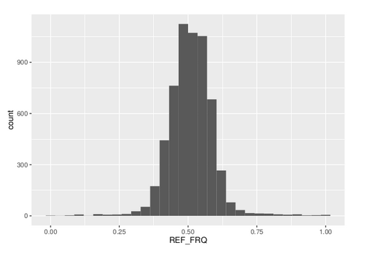
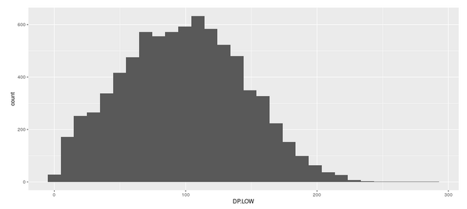
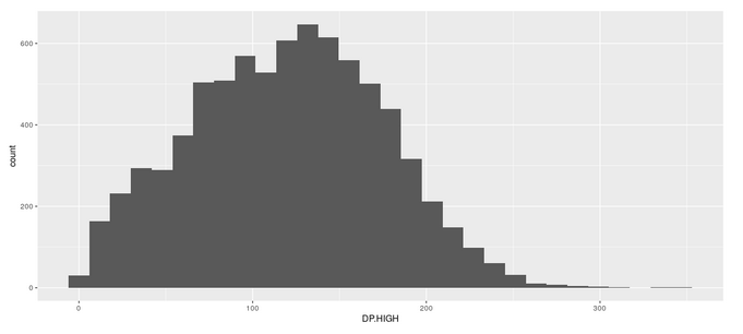
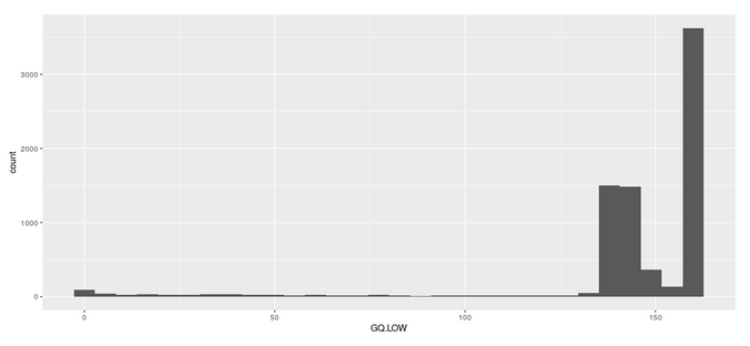
#Plot Depth Distribution
ggplot2::ggplot(data =df) + geom_histogram(aes(x = DP.LOW + DP.HIGH)) + xlim(0,400)


#The plot reveals a skewed G Prime statistic with a really small variance. Perhaps it is due to the small number of variants called.
#In addition, Hampels outlier filter in the second argument, can also be changed to "deltaSNP"
QTLseqr::plotGprimeDist(SNPset = df_filt, outlierFilter = "Hampel")
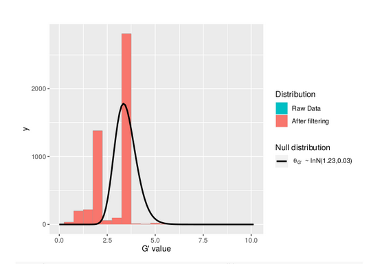
#We can see raw data before and after our filtering step
QTLseqr::plotGprimeDist(SNPset = df_filt, outlierFilter = "deltaSNP",filterThreshold = 0.1)

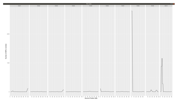
#Plot Snps as a function of chromosome and position values
QTLseqr::plotQTLStats(SNPset = df_filt, var = "nSNPs")
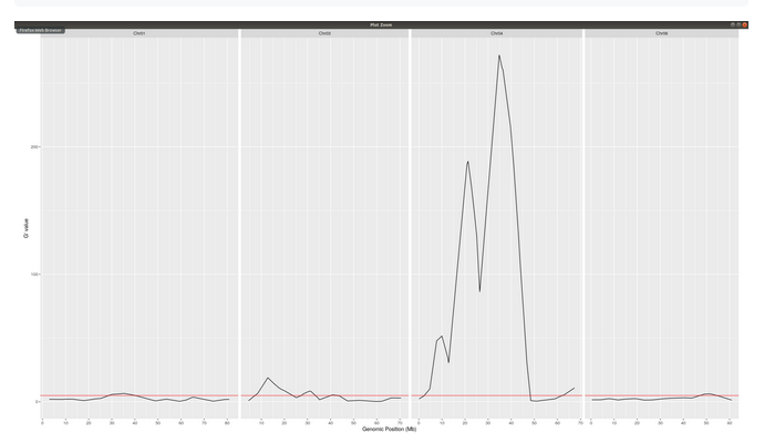
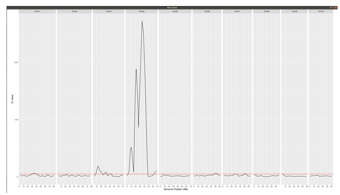
#Using QTLStats funciton plot Gprime Statistic with False Discovery Rate Threhshold as a third argument boolean operator as TRUE. The q value is used as FDR threshold null value is 0.05%.
QTLseqr::plotQTLStats(SNPset = df_filt, var = "Gprime", plotThreshold = TRUE, q = 0.01)
ggplot2::ggsave(filename = "GPrime.png",plot = last_plot())
#Again using plotQTLStats change second argument varaible to deltaSNP and plot.
QTLseqr::plotQTLStats(SNPset = df_filt, var = "deltaSNP", plotIntervals  = TRUE)
ggplot2::ggsave(filename = "DeltaSNPInterval.png",plot = last_plot())
#Add subset argument to focus on particular chromosomes one, three, four, and six.
#The reason is due to signficant QTL regions
QTLseqr::plotQTLStats(SNPset = df_filt, var = "Gprime",plotThreshold = TRUE,q=0.01,subset = c("Chr01","Chr03","Chr04","Chr06"))